Become an Excel pro! 🚀 You can find many related examples and features on the right side of each chapterat the bottom of each chapter. Check out 270 popular pages below.
1 Drop-down List: Drop-down lists in Excel are helpful if you want to be sure that users select an item from a list, instead of typing their own values.

2 Find Duplicates: This page teaches you how to find duplicate values (or triplicates) and how to find duplicate rows in Excel.
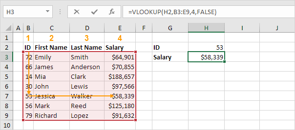
3 Vlookup: The VLOOKUP function is one of the most popular functions in Excel. This page contains many easy to follow VLOOKUP examples.
4 Histogram: This example teaches you how to make a histogram in Excel.
5 Regression: This example teaches you how to run a linear regression analysis in Excel and how to interpret the Summary Output.
6 Percent Change: The percent change formula is used very often in Excel. For example, to calculate the Monthly Change and Total Change.
7 Pareto Chart: A Pareto chart combines a column chart and a line graph. The Pareto principle states that, for many events, roughly 80% of the effects come from 20% of the causes.
8 Loan Amortization Schedule: This example teaches you how to create a loan amortization schedule in Excel.
9 Random Numbers: Excel has two very useful functions when it comes to generating random numbers. RAND and RANDBETWEEN.
10 If: The IF function is one of the most used functions in Excel. This page contains many easy to follow IF examples.
11 Remove Duplicates: This example teaches you how to remove duplicates in Excel.

12 Lock Cells: You can lock cells in Excel if you want to protect cells from being edited.
13 Standard Deviation: This page explains how to calculate the standard deviation based on the entire population using the STDEV.P function in Excel and how to estimate the standard deviation based on a sample using the STDEV.S function in Excel.
14 Count Unique Values: This example shows you how to create an array formula that counts unique values.
15 Gantt Chart: Excel does not offer Gantt as a chart type, but it's easy to create a Gantt chart by customizing the stacked bar chart type.
16 Countif: The powerful COUNTIF function in Excel counts cells based on one criteria. This page contains many easy to follow COUNTIF examples.
17 Budget: This example shows you how to create a budget in Excel. Follow this step-by-step guide and take control of your finances.
18 Line Chart: Line charts are used to display trends over time. Use a line chart if you have text labels, dates or a few numeric labels on the horizontal axis.
19 Transpose: Use the 'Paste Special Transpose' option to switch rows to columns or columns to rows in Excel. You can also use the TRANSPOSE function.
20 Compare Two Lists: This page describes how to compare two lists in Excel using conditional formatting and COUNTIF.
21 Sumif: The powerful SUMIF function in Excel sums cells based on one criteria. This page contains many easy to follow SUMIF examples.

22 Time Sheet: This example teaches you how to create a simple timesheet calculator in Excel.
23 Offset: The OFFSET function in Excel returns a cell or range of cells that is a specified number of rows and columns from a cell or range of cells.
24 Pie Chart: Pie charts are used to display the contribution of each value (slice) to a total (pie). Pie charts always use one data series.
25 Data Tables: Instead of creating different scenarios, you can create a data table to quickly try out different values for formulas. You can create a one variable data table or a two variable data table.
26 t-Test: This example teaches you how to perform a t-Test in Excel. The t-Test is used to test the null hypothesis that the means of two populations are equal.
27 Advanced Filter: This example teaches you how to apply an advanced filter in Excel to only display records that meet complex criteria.
28 Frequency Distribution: Did you know that you can use pivot tables to easily create a frequency distribution in Excel? You can also use the Analysis Toolpak to create a histogram.
29 Subtract: There's no SUBTRACT function in Excel. However, there are many ways to subtract numbers in Excel. Are you ready to improve your Excel skills?
30 Anova: This example teaches you how to perform a single factor ANOVA (analysis of variance) in Excel. A single factor or one-way ANOVA is used to test the null hypothesis that the means of several populations are all equal.
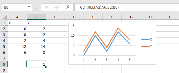
31 Correlation: We can use the CORREL function or the Analysis Toolpak add-in in Excel to find the correlation coefficient between two variables.

32 Compound Interest: What's compound interest and what's the formula for compound interest in Excel? This example gives you the answers to these questions.
33 Bar Chart: A bar chart is the horizontal version of a column chart. Use a bar chart if you have large text labels.
34 Concatenate: Use CONCATENATE, CONCAT, TEXTJOIN or the & operator in Excel to concatenate (join) two or more text strings.
35 Freeze Panes: If you have a large table of data in Excel, it can be useful to freeze rows or columns. This way you can keep rows or columns visible while scrolling through the rest of the worksheet.
36 Weighted Average: To calculate a weighted average in Excel, simply use SUMPRODUCT and SUM.
37 Index and Match: Use INDEX and MATCH in Excel and impress your boss. Instead of using VLOOKUP, use INDEX and MATCH. To perform advanced lookups, you'll need INDEX and MATCH.
38 Delete Blank Rows: This example teaches you how to delete blank rows or rows that contain blank cells.
39 Sumproduct: To calculate the sum of the products of corresponding numbers in one or more ranges, use Excel's powerful SUMPRODUCT function.
40 Merge Cells: Merge cells into one large cell to make clear that a label in Excel applies to multiple columns. Use CONCATENATE, TEXTJOIN or Flash Fill to merge cells without losing data.
41 Scatter Plot: Use a scatter plot (XY chart) to show scientific XY data. Scatter plots are often used to find out if there's a relationship between variables X and Y.

42 Percentage: Calculating percentages in Excel is easy. Percentage simply means 'out of 100', so 72% is '72 out of 100' and 4% is '4 out of 100', etc.
43 Contains Specific Text: To check if a cell contains specific text, use ISNUMBER and SEARCH in Excel. There's no CONTAINS function in Excel.
44 Pmt: The PMT function in Excel calculates the payment for a loan based on constant payments and a constant interest rate. This page contains many easy to follow PMT examples.
45 Calculate Age: To calculate age in Excel, use the DATEDIF function and TODAY. You can also use the age formula to calculate a person’s exact age in years, months, and days.
46 Wrap Text: Wrap text in Excel if you want to display long text on multiple lines in a single cell.
47 Indirect: Use the INDIRECT function in Excel to convert a text string into a valid reference. You can use the & operator to create text strings.
48 Multiply: To multiply numbers in Excel, use the asterisk symbol (*) or the PRODUCT function. Learn how to multiply columns and how to multiply a column by a constant.
49 Subtotal: Use the SUBTOTAL function in Excel instead of SUM, COUNT, MAX, etc. to ignore rows hidden by a filter or to ignore manually hidden rows.
50 Goal Seek: If you know the result you want from a formula, use Goal Seek in Excel to find the input value that produces this formula result.
51 Dynamic Arrays: Dynamic array formulas, entered into a single cell, fill multiple cells. This behavior in Excel 365/2021 is called spilling.

52 CAGR: There's no CAGR function in Excel. However, simply use the RRI function in Excel to calculate the compound annual growth rate (CAGR) of an investment over a period of years.
53 If Cell is Blank: Use the IF function and an empty string in Excel to check if a cell is blank. Use IF and ISBLANK to produce the exact same result.
54 Average: The AVERAGE function in Excel calculates the average (arithmetic mean) of a group of numbers.
55 Substring: There's no SUBSTRING function in Excel. Use MID, LEFT, RIGHT, FIND, LEN, SUBSTITUTE, REPT, TRIM and MAX in Excel to extract substrings.
56 Sum: Use the SUM function in Excel to sum a range of cells, an entire column or non-contiguous cells.
57 Compare Two Columns: To compare two columns, use IF, ISERROR and MATCH in Excel. You can display the duplicates or the unique values.
58 Divide: There's no DIVIDE function in Excel. Simply use the forward slash (/) to divide numbers in Excel.
59 Remove Spaces: The TRIM function in Excel removes leading spaces, extra spaces and trailing spaces. Use the SUBSTITUTE function to remove all spaces or non-breaking spaces.
60 Move Columns: To move columns in Excel, use the shift key or use Insert Cut Cells. You can also change the order of all columns in one magic move.
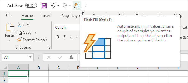
61 Flash Fill: Flash fill is a great Excel tool. Learn how to use flash fill to automatically extract data, combine data, and much more.

62 Hide Columns or Rows: Sometimes it can be useful to hide columns or rows in Excel. Learn how to hide a column, unhide all columns, hide cells, and much more.
63 Check Mark: To insert a check mark symbol in Excel, simply press SHIFT + P and use the Wingdings 2 font. You can also insert a checkbox in Excel.
64 Insert Row: To quickly insert a row in Excel, select a row and use the shortcut CTRL SHIFT +.
65 Comparison Operators: Use comparison operators in Excel to check if two values are equal to each other, if one value is greater than another value, etc.
66 NPV: The correct NPV formula in Excel uses the NPV function to calculate the present value of a series of future cash flows and subtracts the initial investment.
67 Bullet Points: This page illustrates 4 ways to insert bullet points in Excel.
68 AverageIf: The AVERAGEIF function in Excel calculates the average of cells that meet one criteria. AVERAGEIFS calculates the average of cells that meet multiple criteria.
69 Box and Whisker Plot: This example teaches you how to create a box and whisker plot in Excel. A box and whisker plot shows the minimum value, first quartile, median, third quartile and maximum value of a data set.
70 Hyperlinks: Use the 'Insert Hyperlink' dialog box in Excel to create a hyperlink to an existing file, a web page or a place in this document. You can also use the HYPERLINK function.
71 Quick Analysis: Use the Quick Analysis tool in Excel to quickly analyze your data. Quickly calculate totals, quickly insert tables, quickly apply conditional formatting and more.

72 Shade Alternate Rows: To shade alternate rows in Excel, use conditional formatting or apply a table style. Coloring every other row makes it easier to read your data.
73 IRR: Use the IRR function in Excel to calculate a project's internal rate of return.
74 Time Difference: Calculating the difference between two times in Excel can be tricky. Times are handled internally as numbers between 0 and 1.
75 PDF: This page teaches you how to convert an Excel file to a PDF file.
76 Today's Date: To enter today's date in Excel, use the TODAY function. To enter the current date and time, use the NOW function.
77 Forecast: The FORECAST.LINEAR function in Excel predicts a future value along a linear trend. The FORECAST.ETS function in Excel predicts a future value using Exponential Triple Smoothing, which takes into account seasonality.
78 Slicers: Use slicers in Excel to quickly and easily filter pivot tables. Connect multiple slicers to multiple pivot tables to create awesome reports.
79 Split Cells: To split the contents of a cell into multiple cells, use the Text to Columns wizard, flash fill or formulas.
80 Calendar: This example describes how to create a calendar in Excel (2025 calendar, 2026 calendar, etc). If you are in a hurry, simply download the Excel file.
81 Sparklines: Sparklines in Excel are graphs that fit in one cell. Sparklines are great for displaying trends. Excel offers three sparkline types: Line, Column and Win/Loss.

82 Xlookup: If you have Excel 365, use XLOOKUP instead of VLOOKUP. The XLOOKUP function is easier to use and has some additional advantages.
83 Square Root: The square root of a number is a value that, when multiplied by itself, gives the number. The SQRT function in Excel returns the square root of a number.
84 Absolute Reference: To create an absolute reference in Excel, add $ symbols to a cell or range reference. This locks the reference. When you copy a formula, an absolute reference never changes.
85 Randomize List: This article teaches you how to randomize (shuffle) a list in Excel.
86 Circular Reference: A circular reference in Excel occurs when a formula directly or indirectly refers to its own cell. This is not possible.
87 Running Total: This page teaches you how to create a running total (cumulative sum) in Excel. A running total changes each time new data is added to a list.
88 AutoFit: You probably know how to change the width of a column in Excel, but do you also know how to automatically fit the widest entry in a column?
89 Dependent Drop-down Lists: This example describes how to create dependent drop-down lists in Excel.
90 Add or Subtract Time: Use the TIME function in Excel to add or subtract hours, minutes and seconds. To add up times in Excel, simply use the SUM function.
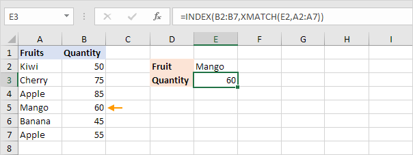
91 Xmatch: The XMATCH function in Excel enhances the MATCH function by adding new features, making it ideal for finding the position of items within arrays or cell ranges.

92 Frequency: The FREQUENCY function in Excel calculates how often values occur within the ranges you specify in a bin table.
93 Trendline: This example teaches you how to add a trendline to a chart in Excel.
94 Not Equal To: In Excel, <> means not equal to. The <> operator in Excel checks if two values are not equal to each other. Let's take a look at a few examples.
95 Weekdays: Use WEEKDAY, NETWORKDAYS and WORKDAY to create cool weekday formulas in Excel. Are you ready to improve your Excel skills?
96 AutoFill: Use AutoFill in Excel to automatically fill a series of cells. This page contains many easy to follow AutoFill examples.
97 Entire Rows and Columns: This example teaches you how to select entire rows and columns in Excel VBA. Are you ready?
98 Combination Chart: A combination chart is a chart that combines two or more chart types in a single chart.
99 Copy a Formula: Simply use CTRL + c and CTRL + v to copy and paste a formula in Excel. Use the fill handle in Excel to quickly copy a formula to other cells.
100 Rank: The RANK function in Excel returns the rank of a number in a list of numbers. Use RANK.AVG to return the average rank if more than one number has the same rank.
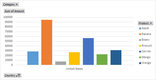
101 Pivot Chart: A pivot chart is the visual representation of a pivot table in Excel. Pivot charts and pivot tables are connected with each other.

102 Lambda: Use LAMBDA and the Name Manager in Excel to create your own Excel function. You can use this custom function like any other Excel function!
103 Show Formulas: By default, Excel shows the results of formulas. To show the formulas instead of their results, press CTRL + ` (you can find this key above the tab key).
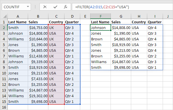
104 FILTER function: Use the magic FILTER function in Excel 365/2021 to extract records that meet certain criteria. The FILTER function is quite versatile.
105 Icon Sets: Icon Sets in Excel make it very easy to visualize values in a range of cells. Each icon represents a range of values.
106 Fractions: This example teaches you how to enter a fraction in Excel and how to change the format of a fraction.
107 Days between Dates: To calculate the number of days between two dates in Excel, subtract the start date from the end date, use DAYS or use DATEDIF.
108 Moving Average: Let's calculate the moving average of a time series in Excel. A moving average is used to smooth out irregularities (peaks and valleys) to easily recognize trends.
109 And: The AND function in Excel evaluates multiple conditions and returns TRUE only if all conditions are TRUE.
110 Day of the Year: An easy formula that returns the day of the year for a given date. There's no built-in function in Excel that can do this.
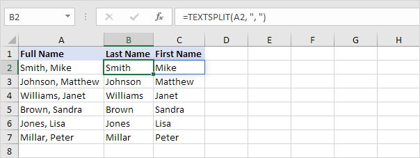
111 TextSplit: Use the TEXTSPLIT function in Excel 365 to split text into rows or columns using delimiters.

112 Reverse List: This article teaches you how to reverse the order of a list in Excel. For example, we want to reverse the list in column A.
113 Delete Row: To quickly delete a row in Excel, select a row and use the shortcut CTRL - (minus sign).
114 BMI calculator: Create a BMI calculator in Excel and find out if you are a healthy weight. Body mass index (BMI) is a measure of body fat based on weight and height that applies to adult men and women.
115 Formula Bar: The formula bar in Excel displays the value or formula of the active cell. You can use the formula bar to enter or edit formulas.
116 Superscript and Subscript: It's easy to format a character as superscript (slightly above the baseline) or subscript (slightly below the baseline) in Excel.
117 Strikethrough: This example teaches you how to apply strikethrough formatting in Excel. You can still read text with a strikethrough effect.
118 Skip Blanks: Use the 'Paste Special Skip Blanks' option and Excel will not overwrite existing values with blanks. To create a formula that skips blank cells, use IF and ISBLANK.
119 Error Bars: This page teaches you how to quickly add error bars to a chart in Excel, followed by instructions for adding custom error bars.
120 Text to Columns: To separate the contents of one Excel cell into separate columns, you can use the 'Convert Text to Columns Wizard'.
121 Sort by Date: This guide walks you through the steps to sort by date in Excel. It starts with how to convert text-formatted dates to actual date values, followed by basic sorting methods and advanced techniques like sorting dates by month and sorting birthdays.

122 Heat Map: To create a heat map in Excel, simply use conditional formatting. A heat map is a graphical representation of data where individual values are represented as colors.
123 Discount: If you know the original price and the discounted price, you can calculate the percentage discount. If you know the original price and the percentage discount, you can calculate the discounted price, etc.
124 Search Box: This example teaches you how to create your own search box in Excel.
125 Kg to lbs: 1 kg = 2.20462 lbs (pounds) and 1 lb (pound) = 0.45359 kg. Use a simple formula, the CONVERT function or download our free unit converter to convert from kg to lbs or vice versa.
126 DateDif: To calculate the number of days, months or years between two dates in Excel, use the DATEDIF function. The DATEDIF function has three arguments.
127 Dynamic Named Range: A dynamic named range expands automatically when you add a value to the range.
128 Background Colors: Changing background colors in Excel VBA is easy. Use the Interior property to return an Interior object. Then use the ColorIndex property of the Interior object to set the background color of a cell.
129 Read-only Workbook: This example shows you how to make your Excel workbook read-only.
130 Last Day of the Month: To get the date of the last day of the month in Excel, use the EOMONTH (End of Month) function.
131 Absolute Value: The ABS function in Excel returns the absolute value of a number. In other words: the ABS function removes the minus sign (-) from a negative number, making it positive.

132 System of Linear Equations: This example shows you how to solve a system of linear equations in Excel.
133 Even and Odd: Use EVEN and ODD in Excel to round numbers. Use ISEVEN or ISODD in Excel to determine if a number is even or odd.
134 Alphabetize: While sorting data alphabetically in Excel is easy, certain situations may require more advanced techniques to achieve the desired alphabetical order.
135 Locate Maximum Value: To find the maximum value in Excel, use the MAX function. To find the cell address of the maximum value in a column, use MAX, MATCH and ADDRESS.
136 IfError: Use the IFERROR function in Excel to return an alternative result, such as text, when a formula evaluates to an error.
137 Two-way Lookup: To lookup a value in a two-dimensional range, use INDEX and MATCH in Excel.
138 Progress Indicator: Learn how to create a progress indicator in Excel VBA. We've kept the progress indicator as simple as possible, yet it looks professional. Are you ready?
139 Most Frequently Occurring Word: This example teaches you how to find the most frequently occurring word in Excel.
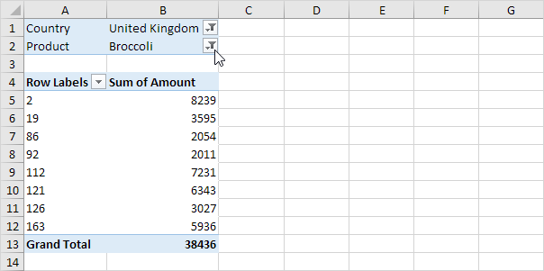
140 GetPivotData: To quickly enter a GETPIVOTDATA function in Excel, type an equal sign (=) and click a cell in a pivot table. The GETPIVOTDATA function can be quite useful.
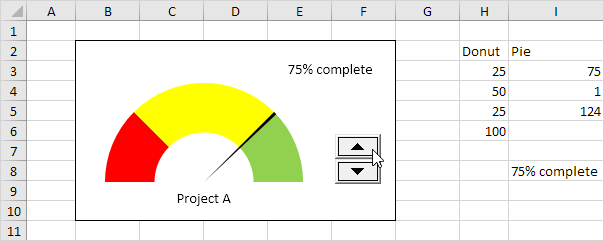
141 Gauge Chart: A gauge chart (or speedometer chart) combines a Doughnut chart and a Pie chart in a single chart. If you are in a hurry, simply download the Excel file.

142 Count Words: Use TRIM, LEN, SUBSTITUTE and SUMPRODUCT in Excel to count words. For example, let's count how many times a specific word occurs in a cell. This trick is pretty cool.
143 Scroll Lock: When Scroll Lock is turned on, you can use the arrow keys to scroll through the worksheet without changing the active cell. Excel displays Scroll Lock in the status bar.
144 Named Range: Create a named range or a named constant and use these names in your Excel formulas. This way you can make your formulas easier to understand.
145 Count Characters: Use the LEN function to count characters in Excel. Use LEN and SUBSTITUTE to count specific characters in Excel.
146 InStr: Use InStr in Excel VBA to find the position of a substring in a string. The InStr function is quite versatile.
147 Merge Tables: You can use tables and the VLOOKUP function in Excel to quickly merge two tables. This trick will bring your Excel game to a new level.
148 Count Errors: This example shows you how to create an array formula that counts the number of errors in a range.
149 XML: Convert your XML file to an Excel file, or vice versa. This enables you to exchange data between different applications.
150 Chart Sheet: You can find most charts on the same worksheet as the source data (embedded charts). However, you can also move a chart to a separate sheet that only contains a chart (chart sheet).
151 Most Used Functions: Let's check out the 10 most used Excel functions. Visit our section about functions for detailed explanations and more awesome functions.

152 Function Keys: Function keys in Excel allow you to do things with your keyboard instead of your mouse to increase your speed.
153 Count Blank/Nonblank Cells: This example shows you how to count blank and nonblank cells in Excel.
154 Formula to Value: To quickly convert a formula to a value in Excel or to convert multiple formulas to values, execute the following steps.
155 Percentiles and Quartiles: This example teaches you how to use PERCENTILE and QUARTILE in Excel.
156 Exponential Smoothing: Exponential smoothing is used to smooth out irregularities (peaks and valleys) to easily recognize trends.
157 Count Cells with Text: This page illustrates multiple ways to count cells with text in Excel. Visit our page about the COUNTIF function to count cells that contain specific text.
158 Depreciation: Excel offers five different depreciation functions. We consider an asset with an initial cost of $10,000, a salvage value (residual value) of $1000 and a useful life of 10 periods (years).
159 Page Numbers: This example teaches you how to insert page numbers in Excel.
160 Column Chart: Column charts are used to compare values across categories by using vertical bars. To create a column chart, execute the following steps.
161 Prevent Duplicate Entries: To prevent duplicate values from being entered into Excel, use data validation and the COUNTIF function.

162 Wildcards: Excel has 3 wildcards. A question mark (?) matches exactly one character. An asterisk (*) matches zero or more characters. And a tilde (~).
163 Negative Numbers to Zero: A clever Excel trick to change negative numbers to zero but leave positive numbers unchanged.
164 Loop through Defined Range: Use Excel VBA to loop through a defined range. For example, when we want to square the numbers in the range A1:A3.
165 LET function: Use the LET function in Excel 365/2021 to declare variables and assign values (or calculation results) to variables. Next, use these variables in a calculation.
166 Date Filters: This page teaches you how to apply a date filter to only display records that meet certain criteria.
167 Profit Margin: Calculating gross profit margin, operating profit margin and net profit margin in Excel is easy. Simply use the formulas explained on this page.
168 Left Lookup: The VLOOKUP function only looks to the right. To look up a value in any column and return the corresponding value to the left, simply use INDEX and MATCH.
169 F-Test: This example teaches you how to perform an F-Test in Excel. The F-Test is used to test the null hypothesis that the variances of two populations are equal.
170 SORT function: Use the magic SORT function in Excel 365/2021 to sort your Excel data by one column or multiple columns. Let's give it a try.
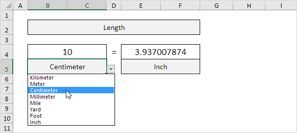
171 Cm to inches: 1 cm = 0.3937 inch and 1 inch = 2.54 cm. Use a simple formula, the CONVERT function or download our free unit converter to convert from cm to inches or vice versa.

172 Color Scales: Color Scales in Excel make it very easy to visualize values in a range of cells. The shade of the color represents the value in the cell.
173 AutoRecover: Excel periodically saves a copy of your Excel file. Learn how to recover a file that was never saved and how to recover a file that has been saved at least once.
174 Descriptive Statistics: You can use the Analysis Toolpak add-in to generate descriptive statistics. For example, you may have the scores of 14 participants for a test.
175 Two-column Lookup: This example teaches you how to perform a two-column lookup in Excel.
176 Get Sheet Name: To return the sheet name in a cell, use CELL, FIND and MID in Excel. There's no built-in function in Excel that can get the sheet name.
177 Rounding Times: Use MROUND in Excel to round a time to the nearest 15 minutes, the nearest 30 minutes, the nearest hour, etc.
178 Protect Sheet: When you share an Excel file with other users, you may want to protect a worksheet to help prevent it from being changed.
179 Axes: Most chart types have two axes: a horizontal axis (or x-axis) and a vertical axis (or y-axis). This example teaches you how to change the axis type, add axis titles and how to change the scale of the vertical axis.
180 Consolidate: You can use Excel's Consolidate feature to consolidate your worksheets (located in one workbook or multiple workbooks) into one worksheet.
181 Multi-level Pivot Table: You can drag more than one field to an area in a pivot table. We'll look at an example of multiple row fields, multiple value fields and multiple report filter fields.

182 InputBox Function: You can use the InputBox function in Excel VBA to prompt the user to enter a value.
183 Sensitivity Analysis: Sensitivity analysis gives you insight into how the optimal solution changes when you change the coefficients of the model. After the solver found a solution, you can create a sensitivity report.
184 Closest Match: To find the closest match to a target value in a data column, use INDEX, MATCH, ABS and MIN in Excel. Use the VLOOKUP function in Excel to find an approximate match.
185 Unique Values: To find unique values in Excel, use the Advanced Filter. You can extract unique values or filter for unique values. If you have Excel 365 or Excel 2021, use the magic UNIQUE function.
186 Import Access Data: This example teaches you how to import data from a Microsoft Access database. In Excel, when you import data, you make a permanent connection that can be refreshed.
187 Paste Special: Use the shortcut Ctrl + Alt + V to display the Paste Special dialog box in Excel. Next, press an underlined letter to paste formulas, values, formatting, etc.
188 Add a Column: To add a column in Excel, right-click the column letter and click Insert. When you insert a column or row, cell references update automatically.
189 Or: The OR function in Excel returns TRUE if any of the conditions are true and returns FALSE if all conditions are false. Combine the OR function with other functions and become an Excel expert.
190 Compare Text: This example shows two ways to compare text strings in Excel. One is case-sensitive and one is case-insensitive.
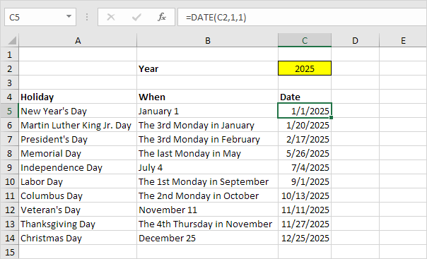
191 Holidays: This example teaches you how to get the date of a holiday for any year (2025, 2026, etc).

192 Custom Sort Order: You can use Excel to sort data in a custom order. In this example, we would like to sort by Priority (High, Normal, Low).
193 Page Breaks: Insert a page break in Excel to specify where a new page will begin in the printed copy.
194 Quadratic Equation: A quadratic equation is of the form ax2 + bx + c = 0 where a ≠ 0. A quadratic equation can be solved by using the quadratic formula. You can also use Excel's Goal Seek feature to solve a quadratic equation.
195 Merge Excel Files: To merge Excel files into one, use the 'Move or Copy' feature. If you need to merge many Excel files, consider using VBA to automate the process.
196 Automated Invoice: This article describes how to automate the generation of invoices in Excel.
197 Online: You can edit Excel files with Excel Online from anywhere without having Excel installed on your computer.
198 Vlookup: Use the WorksheetFunction property in Excel VBA to access the VLOOKUP function. All you need is a single code line.
199 Array Manipulation: Use the new array manipulation functions in Excel 365 to quickly combine, shape and resize arrays.
200 Formula Auditing: Formula auditing in Excel allows you to display the relationship between formulas and cells. The example below helps you master Formula Auditing quickly and easily.
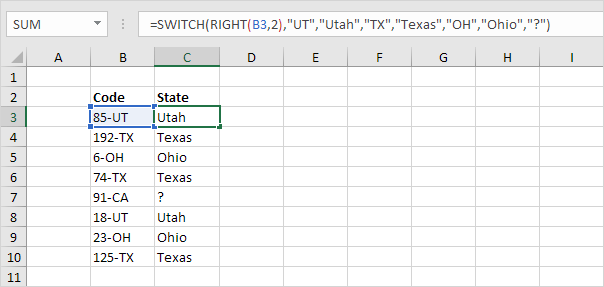
201 Switch: The SWITCH function in Excel looks up a specified value in a list of values and returns the result corresponding to the first match found.

202 Text to Numbers: In Excel, text is left-aligned and numbers are right-aligned. This example teaches you how to convert 'text strings that represent numbers' to numbers.
203 Sum Range with Errors: This example shows you how to create an array formula that sums a range with errors. You can also use the AGGREGATE function to sum a range with errors.
204 Unhide Sheets: Unhiding sheets in Excel is easy. A workbook must contain at least one visible worksheet.
205 User Defined Function: Excel has a large collection of functions. In most situations, those functions are sufficient to get the job done. If not, you can use Excel VBA to create your own function.
206 Zoom in and out: In most cases, you can use the minus and plus symbols in the status bar to quickly zoom the document. Use the buttons on the View tab to zoom to a specific percentage and to zoom to a selection.
207 Quarter Formula: An easy formula that returns the quarter for a given date. There's no built-in function in Excel that can do this.
208 Maximum Flow Problem: Use the solver in Excel to find the maximum flow from node S to node T in a directed network.
209 Separate Strings: To separate strings in Excel, use RIGHT, LEN, FIND and LEFT. If you're not a formula hero, use Flash Fill to split text strings in Excel.
210 MaxIfs and MinIfs: Use MAXIFS and MINIFS in Excel to find the maximum and minimum value based on one criteria or multiple criteria.
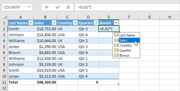
211 Structured References: When working with tables in Excel, you can use structured references to make your formulas easier to understand.

212 Currency Converter: Use Excel VBA to create a Userform that converts any amount from one currency into another.
213 IsError: This example illustrates the ISERROR function in Excel.
214 Date and Time Formats: Dates and times in Excel can be displayed in a variety of ways. To apply a Date or Time format, execute the following steps.
215 Comments: Insert a comment in Excel to start a conversation or to give feedback about the content of a cell. Old style comments are still available and are now called notes.
216 Sum Largest Numbers: To sum the largest numbers in an Excel range, create an array formula or simply combine the SUMIF function with the LARGE function.
217 Case-sensitive Lookup: By default, the VLOOKUP function performs a case-insensitive lookup. However, you can use INDEX, MATCH and EXACT in Excel to perform a case-sensitive lookup.
218 Calculated Field/Item: This example teaches you how to insert a calculated field or calculated item in a pivot table.
219 Days until Birthday: To calculate the number of days until your birthday in Excel, execute the following steps.
220 Name Box: You can use the name box in Excel to select a cell, range or named range. You can also use the name box to quickly create a named range (important).
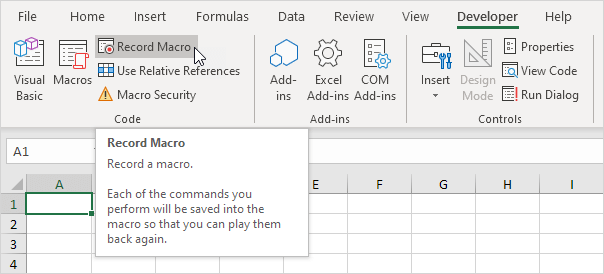
221 Macro Recorder: The Macro Recorder, a very useful tool included in Excel VBA, records every task you perform with Excel. All you have to do is record a specific task once. Next, you can execute the task over and over with the click of a button.

222 Custom Number Format: Excel has many built-in formats that you can use: Currency, Accounting, Date, Time, Percentage, etc. If you cannot find the right format, you can create a custom number format.
223 ROW function: The ROW function in Excel returns the row number of a reference. For example, =ROW(C4) returns 4. The ROW function can be quite useful.
224 Format Painter: The Format Painter is one of the most underused features of Excel. The Format Painter copies formatting from one place and applies it to another.
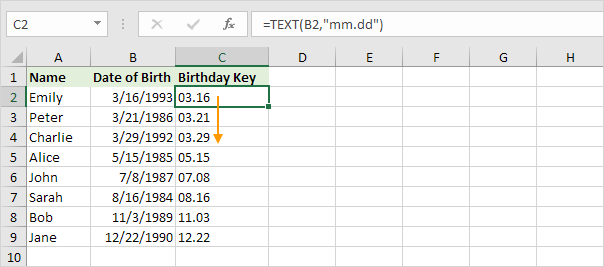
225 Text: When joining text and a number, use the TEXT function in Excel to format that number. This page contains many easy to follow TEXT function examples.
226 Assignment Problem: Use the solver in Excel to find the assignment of persons to tasks that minimizes the total cost.
227 Custom Lists: If you create a custom list in Excel, you can easily fill a range with your own list of departments, clients, cities, credit card numbers, etc. This can save time and reduce errors.
228 Highlight Active Cell: Learn how to create a program in Excel VBA that highlights the row and column of the Active Cell (selected cell). This program will amaze and impress your boss.
229 Spell Check: Learn how to check the spelling of text in Excel, add words to your custom dictionary (or AutoCorrect list) and learn how to change spell checking options.
230 Copy Visible Cells Only: By default, Excel copies both visible and hidden cells. However, it is possible to copy visible cells only.
231 Quick Access Toolbar: If you use an Excel command frequently, you can add it to the Quick Access Toolbar. By default, the Quick Access Toolbar contains four commands: AutoSave, Save, Undo and Redo.

232 Data Form: The data form in Excel allows you to add, edit and delete records (rows) and display only those records that meet certain criteria. Especially when you have wide rows and you want to avoid repeated scrolling to the right and left, the data form can be useful.
233 Find: Use the FIND function in Excel to find the position of a substring in a string. The FIND function is case-sensitive.
234 OneDrive: Save your Excel files to your OneDrive location and access your files from any computer or share them with other people.
235 Table as Source Data: One of the great things about tables in Excel is that you can use a table as source data for a chart, pivot table, etc.
236 Check Box: A check box is a field which can be checked to store information. To create a check box in Excel VBA, execute the following steps.
237 Default Templates: Book.xltx and Sheet.xltx are two special templates you can create and add to the XLStart folder. As a result, Excel uses Book.xltx as the basis for new workbooks and Sheet.xltx as the basis for new worksheets.
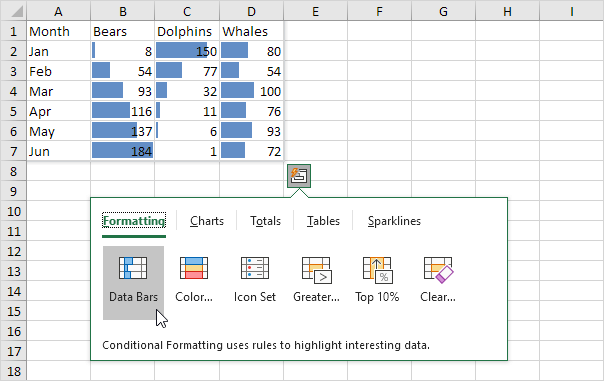
238 Data Bars: Data bars in Excel make it very easy to visualize values in a range of cells. A longer bar represents a higher value.
239 Read Data from Text File: Use Excel VBA to read data from a text file. This file contains some geographical coordinates we want to import into Excel.
240 Aggregate: Excel functions such as SUM, COUNT, LARGE and MAX don't work if a range includes errors. However, you can easily use the AGGREGATE function to fix this.
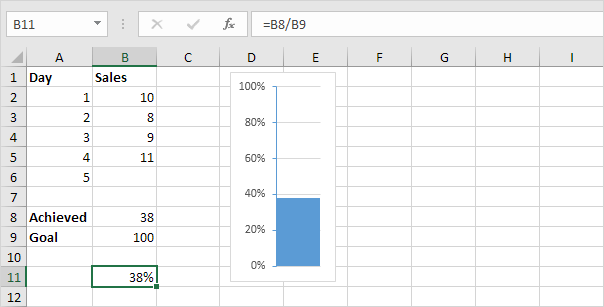
241 Thermometer Chart: This example teaches you how to create a thermometer chart in Excel. A thermometer chart shows you how much of a goal has been achieved.

242 Table Styles: Quickly format a range of cells by choosing a table style. You can also create your own table style.
243 Status Bar: The status bar in Excel can be quite useful. By default, the status bar at the bottom of the window displays the average, count and sum of selected cells.
244 Import Sheets: In this example, we will create a VBA macro that imports sheets from other Excel files into one Excel file.
245 Meal Planner: This article shows you how to create a meal planner in Excel. Use drop-down lists to easily select meals for breakfast, lunch, and dinner.
246 Count with Or Criteria:: Counting with Or criteria in Excel can be tricky. This article shows several easy to follow examples.
247 Shortest Path Problem: Use the solver in Excel to find the shortest path from node S to node T in an undirected network. Points in a network are called nodes (S, A, B, C, D, E and T). Lines in a network are called arcs (SA, SB, SC, AC, etc).
248 Chop off Decimals: This example illustrates two functions to chop off decimals in Excel. INT and TRUNC.
249 Group Worksheets: Group worksheets in Excel to edit multiple worksheets at the same time. Our workbook contains 3 similar worksheets (North, Mid and South) and a blank fourth worksheet.
250 Sort by Color: This example teaches you how to sort data by color in Excel.
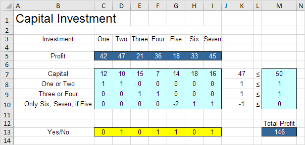
251 Capital Investment: Use the solver in Excel to find the combination of capital investments that maximizes the total profit.

252 Find Features: This page illustrates useful find features in Excel. Learn how to perform workbook-wide searches, case-sensitive searches, find exact cell content, and use wildcards.
253 Invoice: This article describes how to create a simple invoice in Excel.
254 Outlining Data: Outlining data makes your data easier to view. In this example, we will total rows of related data and collapse a group of columns.
255 Row Differences: This example teaches you how to quickly highlight cells whose contents are different from the comparison cell in each row.
256 Add a Macro to the Toolbar: If you use an Excel macro frequently, you can add it to the Quick Access Toolbar. This way you can quickly access your macro.
257 Import/Export Text Files: This article describes how to import or export text files. Text files can be comma separated (.csv) or tab separated (.txt)
258 Themes: Excel offers themes to change the look of your workbook with the click of a button. Each theme consists of 12 colors, two fonts (Headings and Body) and effects for shapes and SmartArt.
259 Group Pivot Table Items: This example teaches you how to group pivot table items. Learn how to group products and how to group dates by quarters.
260 Sum with Or Criteria: Summing with Or criteria in Excel can be tricky. This article shows several easy to follow examples.
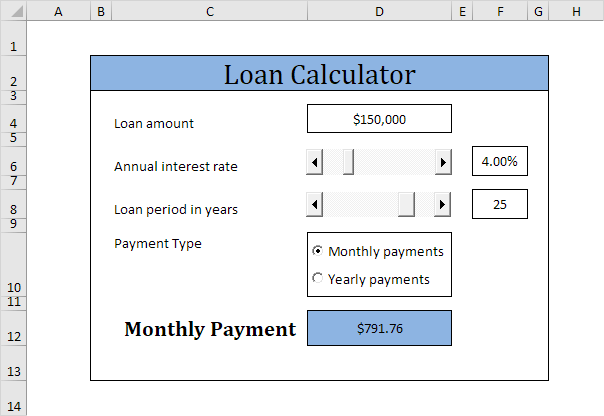
261 Loan Calculator: This page teaches you how to create a simple loan calculator in Excel VBA. The worksheet contains the following ActiveX controls: two scrollbars and two option buttons.

262 Debugging: This example teaches you how to debug code in Excel VBA.
263 Transportation Problem: Use the solver in Excel to find the number of units to ship from each factory to each customer that minimizes the total cost.
264 Paste Options: This example illustrates the various paste options in Excel.
265 Sum Every Nth Row: This example shows you how to create an array formula that sums every nth row in Excel. We will show it for n = 3, but you can do this for any number.
266 Customize the Ribbon: The ribbon in Excel can be customized. You can easily create your own tab and add commands to it.
267 Reject Invalid Dates: This example teaches you how to use data validation to reject invalid dates.
268 Mode: Use the MODE function in Excel to find the most frequently occurring number in a list of numbers. Use MODE.MULT to find multiple modes.
269 Update Pivot Table: Any changes you make to the data set are not automatically picked up by the pivot table. Refresh the pivot table or change the data source to update the pivot table with the applied changes.
270 Number and Text Filters: This example teaches you how to apply a number filter and a text filter to only display records that meet certain criteria.
Check out all 300 examples.


