Hide Columns or Rows in Excel

Sometimes it can be useful to hide columns or rows in Excel. Learn how to hide a column, unhide all columns, hide cells, and much more.

Hide

To hide a column, execute the following steps.

1. Select a column.

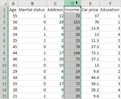
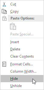
2. Right click, and then click Hide.

Result:

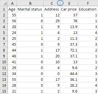
Note: to hide a row, select a row, right click, and then click Hide.

Unhide

To unhide a column, execute the following steps.

1. Select the columns on either side of the hidden column.

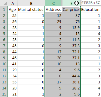
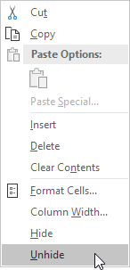
2. Right click, and then click Unhide.

Result:

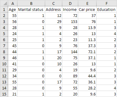
Note: to unhide a row, select the rows on either side of the hidden row, right click, and then click Unhide.

Multiple Columns or Rows

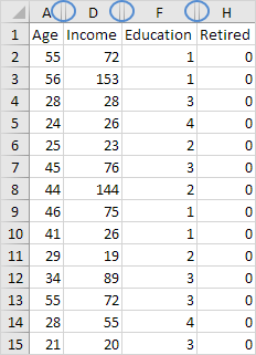
To hide multiple columns, execute the following steps.

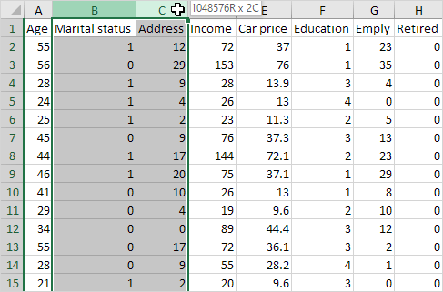
1. Select multiple columns by clicking and dragging over the column headers.

2. To select non-adjacent columns, hold CTRL while clicking the column headers.

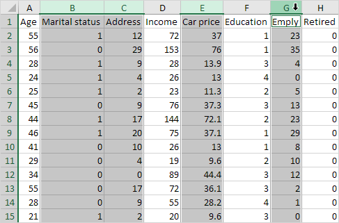
3. Right click, and then click Hide.

Result:

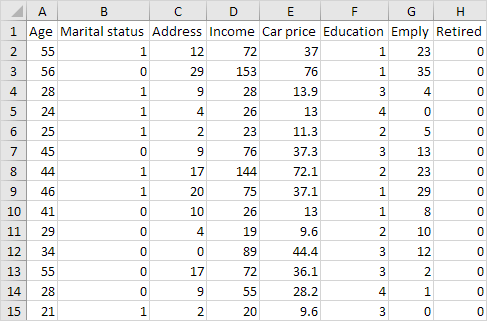
To unhide all columns, execute the following steps.

4. Select all columns by clicking the Select All button.

5. Right click a column header, and then click Unhide.

Result:

Note: in a similar way, you can hide and unhide multiple rows.

Hidden Tricks

Impress your boss with the following hidden :-) tricks. To hide and show columns with the click of a button, execute the following steps.

1. Select one or more columns.

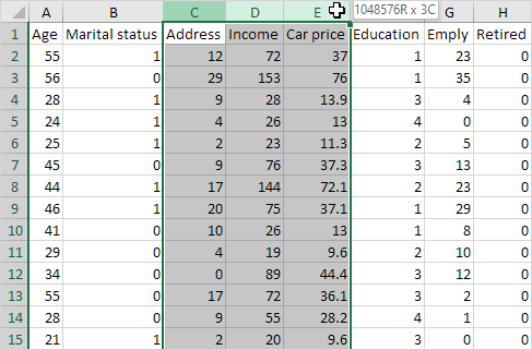
2. On the Data tab, in the Outline group, click Group.

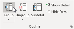
3. To hide the columns, click the minus sign.

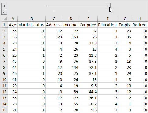
4. To show the columns again, click the plus sign.

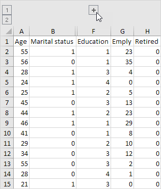
Note: to ungroup the columns, first, select the columns. Next, on the Data tab, in the Outline group, click Ungroup.

Finally, to hide cells in Excel, execute the following steps.

1. Select a range of cells.

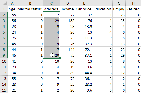
2. Right click, and then click Format Cells.

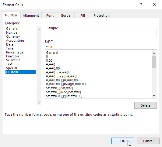
The 'Format Cells' dialog box appears.

3. Select Custom.

4. Type the following number format code: ;;;

5. Click OK.

Result:

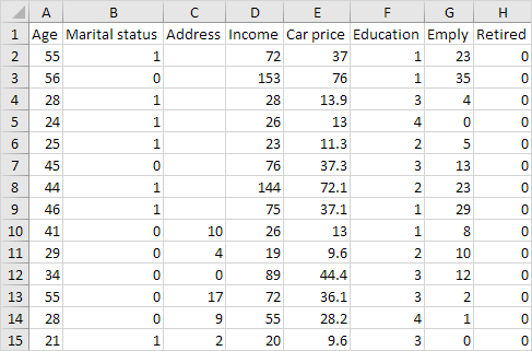
Note: the data is still there. Try it yourself. Download the Excel file, hide cells, select one of the hidden cells and look at the formula bar.