SUBTOTAL function in Excel

Use the SUBTOTAL function in Excel (instead of SUM, COUNT, MAX, etc.) to ignore rows hidden by a filter or to ignore manually hidden rows.

Rows Hidden by a Filter

The SUBTOTAL function ignores rows hidden by a filter, unlike the SUM function, which includes them.

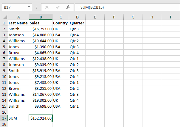
1. For example, the SUM function below calculates the total sales.

2. Apply a filter.

3. The SUM function includes rows hidden by a filter.

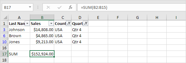
4. The SUBTOTAL function ignores rows hidden by a filter and calculates the correct result.

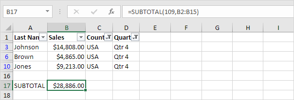
Note: 109 is the argument for Sum if you use the SUBTOTAL function.

5. It's not easy to remember which argument belongs to which function. Fortunately, the AutoComplete feature in Excel helps you with this.

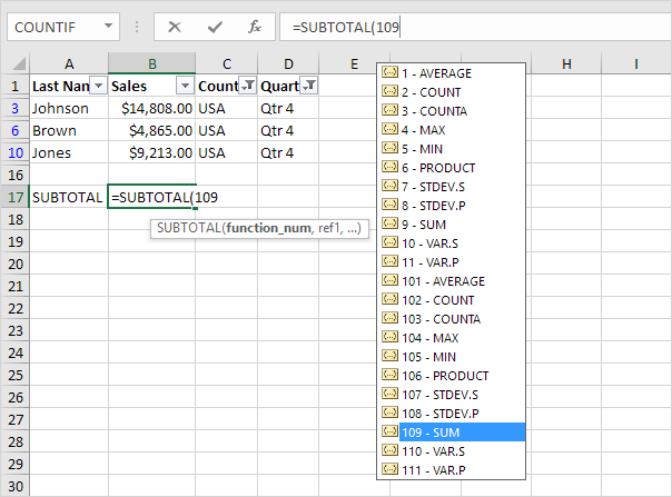
Note: instead of using 101 (AVERAGE) for the first argument, you could also use 1 (AVERAGE), instead of using 102 (COUNT), you could also use 2 (COUNT), etc. When filtering data, there's no difference between the numbers 101-111 and the numbers 1-11.

Manually Hidden Rows

The SUBTOTAL function can ignore manually hidden rows. This is helpful when you manually hide rows but still want an accurate total based on what's visible.

1. For example, the SUM function below sums a range of cells.

2. Hide row 2.

3. The SUM function includes manually hidden rows.

4. The SUBTOTAL function ignores manually hidden rows and calculates the correct result.

Caution: the numbers 101-111 ignore manually hidden rows. However, the numbers 1-11 include manually hidden rows!

Automatic Subtotals

We saved the best for last. Excel can automatically add SUBTOTAL functions for you.

1. The first option. Create a table and add a total row to the bottom of the table. Next, click any cell in the last row to automatically add a SUBTOTAL function.

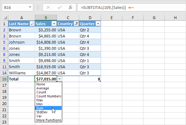
Explanation: in this example, we also filtered by Country. Excel uses the SUBTOTAL function to correctly calculate the total sales in the USA.

2. The second option. On the Data tab, in the Outline group, click Subtotal to outline your data.

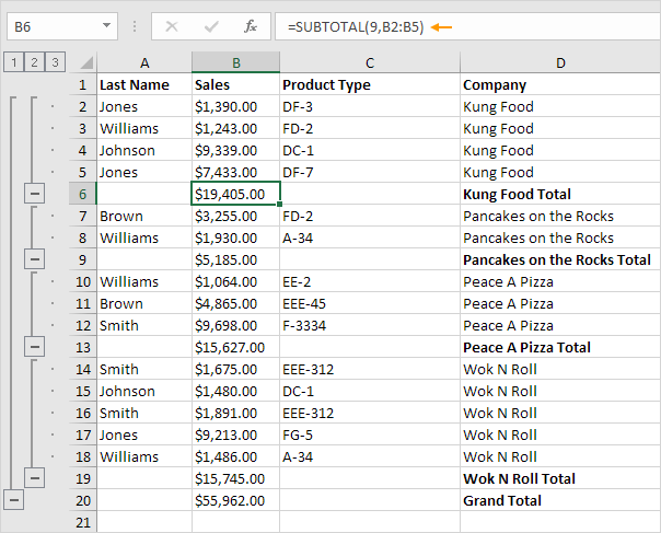
Explanation: in this example, Excel automatically added 5 SUBTOTAL functions (B6, B9, B13, B19 and B20). Follow the link for more information.