Find Duplicates in Excel

This page teaches you how to find duplicate values (or triplicates) and how to find duplicate rows in Excel. It also covers removing duplicates with the Remove Duplicates tool.

Find Duplicate Values

To find and highlight duplicate values in Excel, execute the following steps.

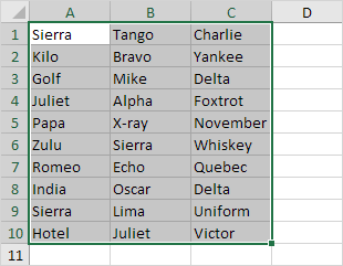
1. Select the range A1:C10.

2. On the Home tab, in the Styles group, click Conditional Formatting.

3. Click Highlight Cells Rules, Duplicate Values.

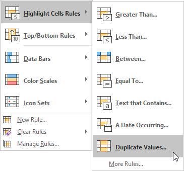
4. Select a formatting style and click OK.

Result: Excel highlights the duplicate names.

Note: select Unique from the first drop-down list to highlight the unique names.

Find Triplicates

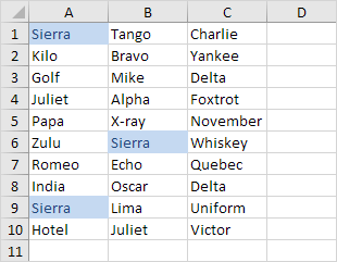
By default, Excel highlights duplicates (Juliet, Delta), triplicates (Sierra), etc. (see previous image). Execute the following steps to highlight triplicates only.

1. First, clear the previous conditional formatting rule.

2. Select the range A1:C10.

3. On the Home tab, in the Styles group, click Conditional Formatting.

4. Click New Rule.

5. Select 'Use a formula to determine which cells to format'.

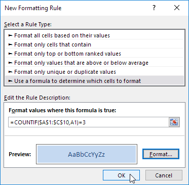
6. Enter the formula =COUNTIF($A$1:$C$10,A1)=3

7. Select a formatting style and click OK.

Result: Excel highlights the triplicate names.

Explanation: =COUNTIF($A$1:$C$10,A1) counts the number of names in the range A1:C10 that are equal to the name in cell A1. If COUNTIF($A$1:$C$10,A1) = 3, Excel formats cell A1. Always write the formula for the upper-left cell in the selected range (A1:C10). Excel automatically copies the formula to the other cells. Thus, cell A2 contains the formula =COUNTIF($A$1:$C$10,A2)=3, cell A3 contains the formula =COUNTIF($A$1:$C$10,A3)=3, etc. Notice how we created an absolute reference ($A$1:$C$10) to lock this reference.

Note: you can use any formula you like. For example, use =COUNTIF($A$1:$C$10,A1)>3 to highlight names that occur more than 3 times.

Find Duplicate Rows

To find and highlight duplicate rows in Excel, use COUNTIFS (with the letter S at the end) instead of COUNTIF.

1. Select the range A1:C10.

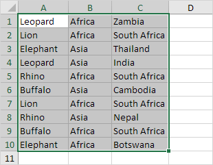
2. On the Home tab, in the Styles group, click Conditional Formatting.

3. Click New Rule.

4. Select 'Use a formula to determine which cells to format'.

5. Enter the formula =COUNTIFS(Animals,$A1,Continents,$B1,Countries,$C1)>1

6. Select a formatting style and click OK.

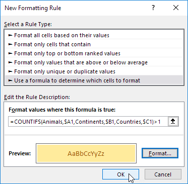
Note: the named range Animals refers to the range A1:A10, the named range Continents refers to the range B1:B10 and the named range Countries refers to the range C1:C10. =COUNTIFS(Animals,$A1,Continents,$B1,Countries,$C1) counts the number of rows based on multiple criteria (Leopard, Africa, Zambia).

Result: Excel highlights the duplicate rows.

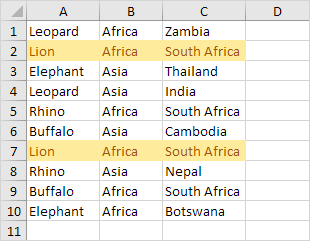
Explanation: if COUNTIFS(Animals,$A1,Continents,$B1,Countries,$C1) > 1, in other words, if there are multiple (Leopard, Africa, Zambia) rows, Excel formats cell A1. Always write the formula for the upper-left cell in the selected range (A1:C10). Excel automatically copies the formula to the other cells. We locked the reference to each column by placing a $ symbol in front of the column letter ($A1, $B1 and $C1). As a result, cell A1, B1 and C1 contain the same formula, cell A2, B2 and C2 contain the formula =COUNTIFS(Animals,$A2,Continents,$B2,Countries,$C2)>1, etc.

Remove Duplicates

Finally, you can use the Remove Duplicates tool in Excel to quickly remove duplicate values or duplicate rows. On the Data tab, in the Data Tools group, click Remove Duplicates.

In the example below, Excel removes all identical rows (blue) except for the first identical row found (yellow).

Note: visit our page about removing duplicates to learn more about this great Excel tool.