OFFSET

Return a Cell | Return a Range | Negative Offset

The OFFSET function in Excel returns a cell or range of cells that is a specified number of rows and columns from a cell or range of cells.

Return a Cell

First, let's use the OFFSET function in Excel to return a cell. Here we go.

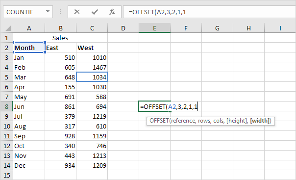
1. The OFFSET function below returns the cell that is 3 rows below and 2 columns to the right of cell A2. The OFFSET function returns a cell because the height and width are both set to 1.

Result:

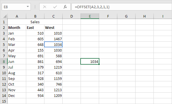
The last 2 arguments of the OFFSET function are optional. When height and width are omitted, the new reference has the same height and width as the starting reference (first argument).

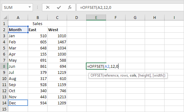
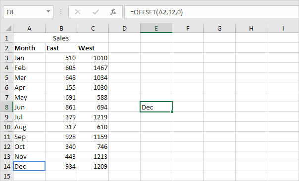
2. For example, the OFFSET function below returns the cell that is 12 rows below and 0 columns to the right of cell A2.

Result:

Return a Range

Alright. Let's now use the OFFSET function in Excel to return a range (two or more cells).

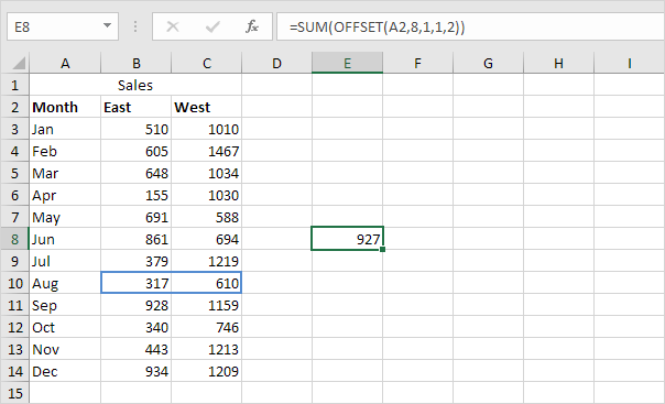
1. The OFFSET function below returns the 1 x 2 range that is 8 rows below and 1 column to the right of cell A2. The SUM function calculates the sum of this range.

Result:

The last 2 arguments of the OFFSET function are optional (as previously mentioned). When height and width are omitted, the new reference has the same height and width as the starting reference (first argument).

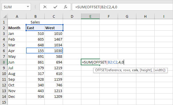
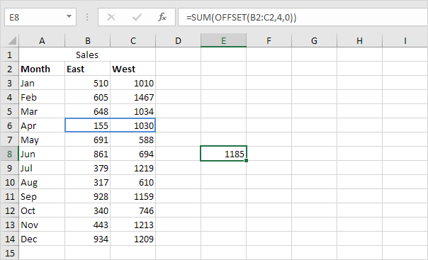
2. For example, the OFFSET function below returns the range that is 4 rows below and 0 columns to the right of the range B2:C2. The SUM function calculates the sum of this range.

Result:

3. The OFFSET function below returns the range that is 4 rows below and 0 columns to the right of the range B2:C2. This time without a SUM function.

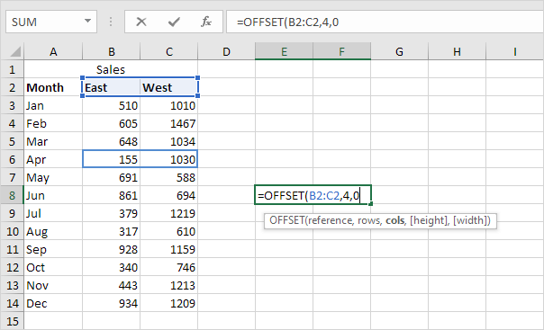
Result:

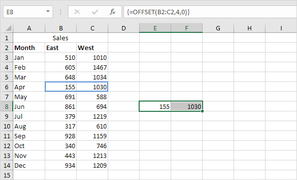
Note: before inserting this formula, select the range E8:F8 (or another range of the same size). Finish by pressing CTRL + SHIFT + ENTER. The formula bar indicates that this is an array formula by enclosing it in curly braces {}. To delete this array formula, select the range E8:F8 and press Delete.

4. If you have Excel 365 or Excel 2021, simply select cell E8, enter the OFFSET function and press Enter. Bye bye curly braces.

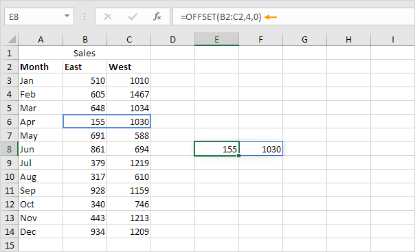
Note: the OFFSET function, entered into cell E8, fills multiple cells. Wow! This behavior in Excel 365/2021 is called spilling.

Negative Offset

If you want to return a cell or range of cells that is a specified number of rows above or columns to the left, use negative numbers.

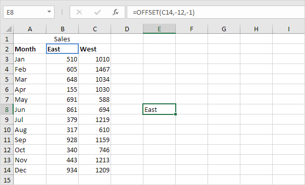
The OFFSET function below returns the cell that is 12 rows above and 1 column to the left of cell C14.

Result: