Group Pivot Table Items in Excel
This example teaches you how to group pivot table items. Learn how to group products and how to group dates by quarters.
Below you can find a pivot table. Go back to Pivot Tables to learn how to create this pivot table.

Group Products
The Product field contains 7 items. Apple, Banana, Beans, Broccoli, Carrots, Mango and Orange.
To create two groups, execute the following steps.
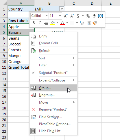
1. In the pivot table, select Apple and Banana.
2. Right click and click on Group.
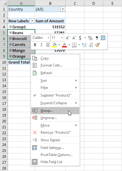
3. In the pivot table, select Beans, Broccoli, Carrots, Mango and Orange.
4. Right click and click on Group.
Result:
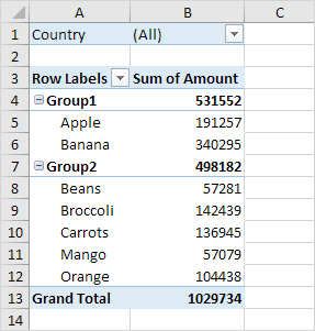
Note: to change the name of a group (Group1 or Group2), select the name, and edit the name in the formula bar. To ungroup, select the group, right click and click on Ungroup.
5. To collapse the groups, click the minus signs.
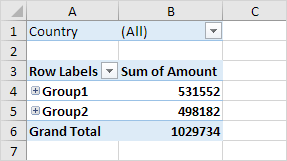
Conclusion: Apple and Banana (Group1) have a higher total than all the other products (Group2) together.
Group Dates
To create the pivot table below, instead of the Product field, add the Date field to the Rows area. The Date field contains many items. 6-Jan, 7-Jan, 8-Jan, 10-Jan, 11-Jan, etc.
To group these dates by quarters, execute the following steps.
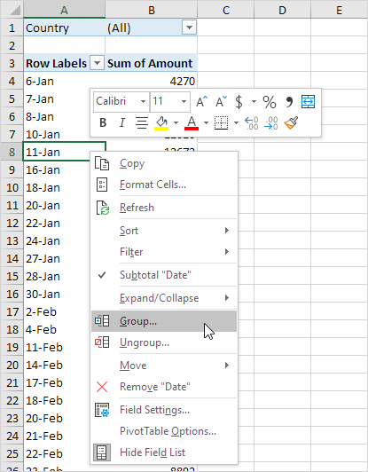
1. Click any cell inside the column with dates.
2. Right click and click on Group.
3. Select Quarters and click OK.
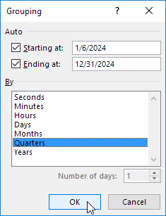
Note: also see the options to group by seconds, minutes, hours, etc.
Result:
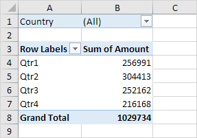
Conclusion: Quarter 2 is the best quarter.