Table Styles in Excel

Quickly format a range of cells by choosing a table style. You can also create your own table style. Quickly format a cell by choosing a cell style.

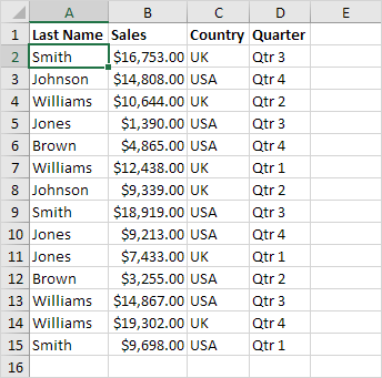
1. Click any single cell inside the data set.

2. On the Home tab, in the Styles group, click Format as Table.

3. Choose a table style.

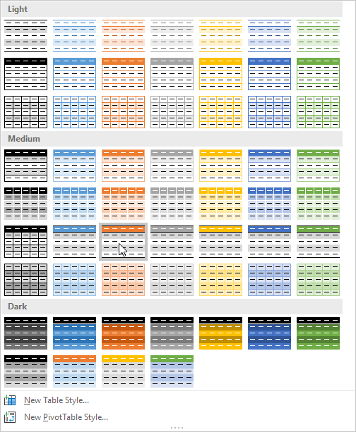
Note: click New Table Style to create your own table style or right click a table style and click Duplicate to create a new table style that is similar to an existing one. Modifying a custom table style affects all tables in a workbook that use that table style. This can save a lot of time.

4. Excel automatically selects the data for you. Check 'My table has headers' and click on OK.

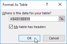
This is another way to create a table. See the result below.

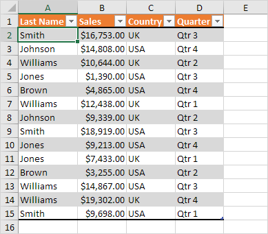
You can change a table style at any time.

5. First, select a cell inside the table. Next, on the Table Design tab, in the Table Styles group, click a table style (hover over a style to see a live preview).

Result: a different visual style.

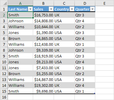
To convert this table back to a normal range of cells (with table formatting), execute the following steps.

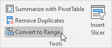
6. First, select a cell inside the table. Next, on the Table Design tab, in the Tools group, click Convert to Range.

Result: a nicely formatted range of cells.

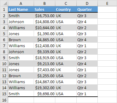
To convert this table back to a normal range of cells (without table formatting), execute the following steps.

7. Press Ctrl + Z to undo the previous step.

8. First, select a cell inside the table. Next, on the Table Design tab, in the Table Styles group, click the first style (None).

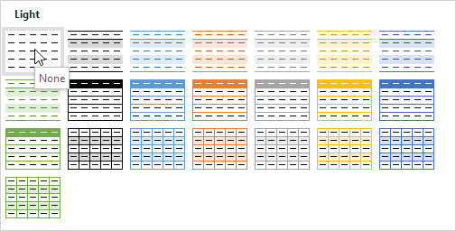
Result: this only removes the table formatting. You can still sort, filter, add a total row, etc.

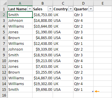
9. Finally, on the Table Design tab, in the Tools group, click Convert to Range.

Result: a normal range of cells.

If you're new here, welcome to Excel Easy! Join over 1 million monthly Excel learners. You can find popular courses here: Excel Functions and Data Analysis in Excel.