Status Bar in Excel

The status bar in Excel can be quite useful. By default, the status bar at the bottom of the window displays the average, count and sum of selected cells.

Status Bar 101

The status bar in Excel can do the math for you.

1. Select the range A1:A3.

2. Look at the status bar to see the average, count and sum of these cells.

3. To quickly change the workbook view, use the 3 view shortcuts on the status bar.

Note: visit our page about workbook views to learn more about this topic.

4. Use the zoom slider on the status bar to quickly zoom in or out to a preset percentage.

Note: use the ribbon to zoom to a specific percentage or to zoom to a selection.

Customize Status Bar

Many status bar options are selected by default. Right click the status bar to activate even more options.

1. Right click the status bar.

2. For example, click Caps Lock.

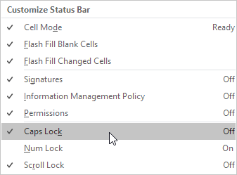
Note: this doesn't turn on Caps Lock (see image above, Caps Lock is still turned off). The status bar displays the Caps Lock status now.

3. Press the Caps Lock key on your keyboard.

4. Excel displays the text Caps Lock in the status bar.

5. Right click the status bar.

6. For example, click Minimum.

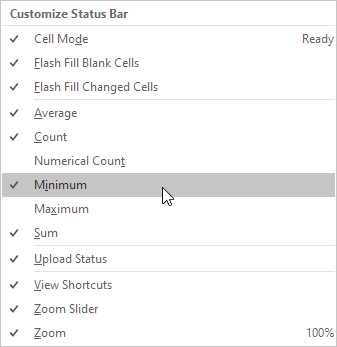
7. Select the range A1:A3.

8. Look at the status bar to see the average, count, minimum and sum of these cells.

Status Bar Secrets

Here's a little secret: Excel uses the status bar in many other situations. If you don't like this, hide the status bar.

1. For example, filter a table.

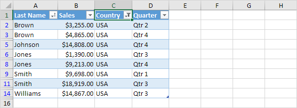
2. Excel uses the status bar to display the number of visible records.

3. Hover over a cell with one or more comments.

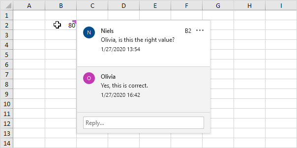
4. Excel uses the status bar to display the name of the author.

5. If you have Excel 2016, use the shortcut CTRL + SHIFT + F1 to hide the ribbon and the status bar.

6. To only hide the status bar, add the following code line to the Workbook Open Event:

7. Use the StatusBar property in Excel VBA to display a message on the status bar.

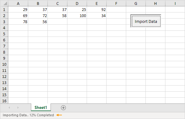
Note: if you're new to Excel, you can skip step 6 and step 7.

If you're new here, welcome to Excel Easy! Join over 1 million monthly Excel learners. You can find popular courses here: Excel Functions and Data Analysis in Excel.