Two-way Lookup in Excel
To lookup a value in a two-dimensional range, use INDEX and MATCH in Excel. Below you can find the sales of different ice cream flavors in each month.
1. To find the position of Feb in the range A2:A13, use the MATCH function. The result is 2.
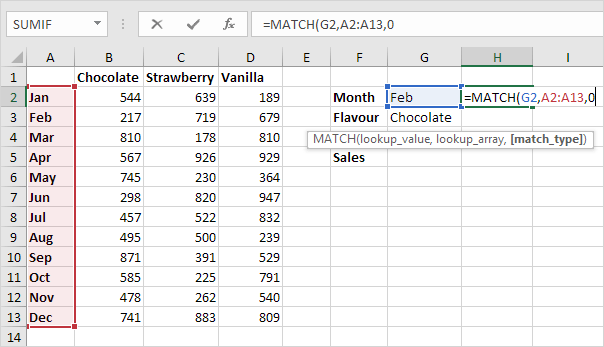
2. To find the position of Chocolate in the range B1:D1, use the MATCH function. The result is 1.

3. Use these results and the INDEX function to find the sales of Chocolate in February.
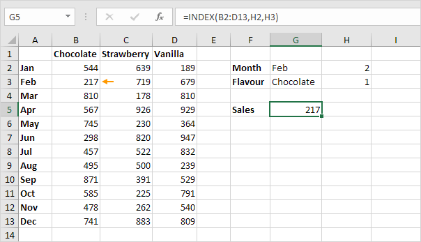
Explanation: 217 found at the intersection of row 2 and column 1 in the range B2:D13.
4. Put it all together.
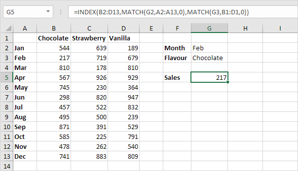
You can also lookup a value in a two-dimensional range without using INDEX and MATCH. The following trick is pretty awesome.
5. Select the range A1:D13.
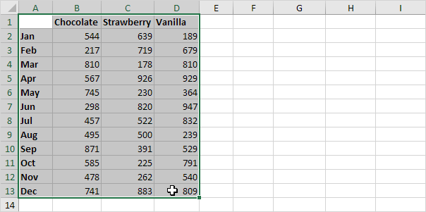
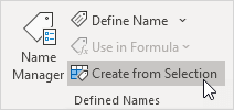
6. On the Formulas tab, in the Defined Names group, click Create from Selection.
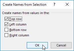
7. Check Top row and Left column and click OK.
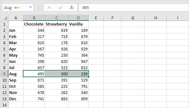
8. Excel created 12 + 3 = 15 named ranges! Simply select a range and look at the Name box.
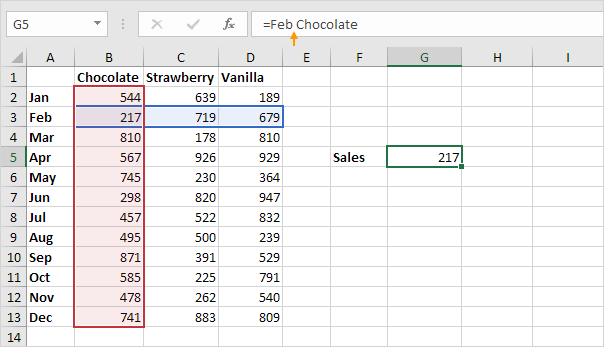
9. Use the intersect operator (space) to return the intersection of two named ranges.
10. Create a dynamic two-way lookup.
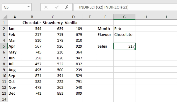
Explanation: the INDIRECT functions convert the text strings ("Feb" in cell G2 and "Chocolate" in cell G3) into valid named ranges.